Build a Hierarchical NeRF with JAX and JAX3D: A Practical Guide

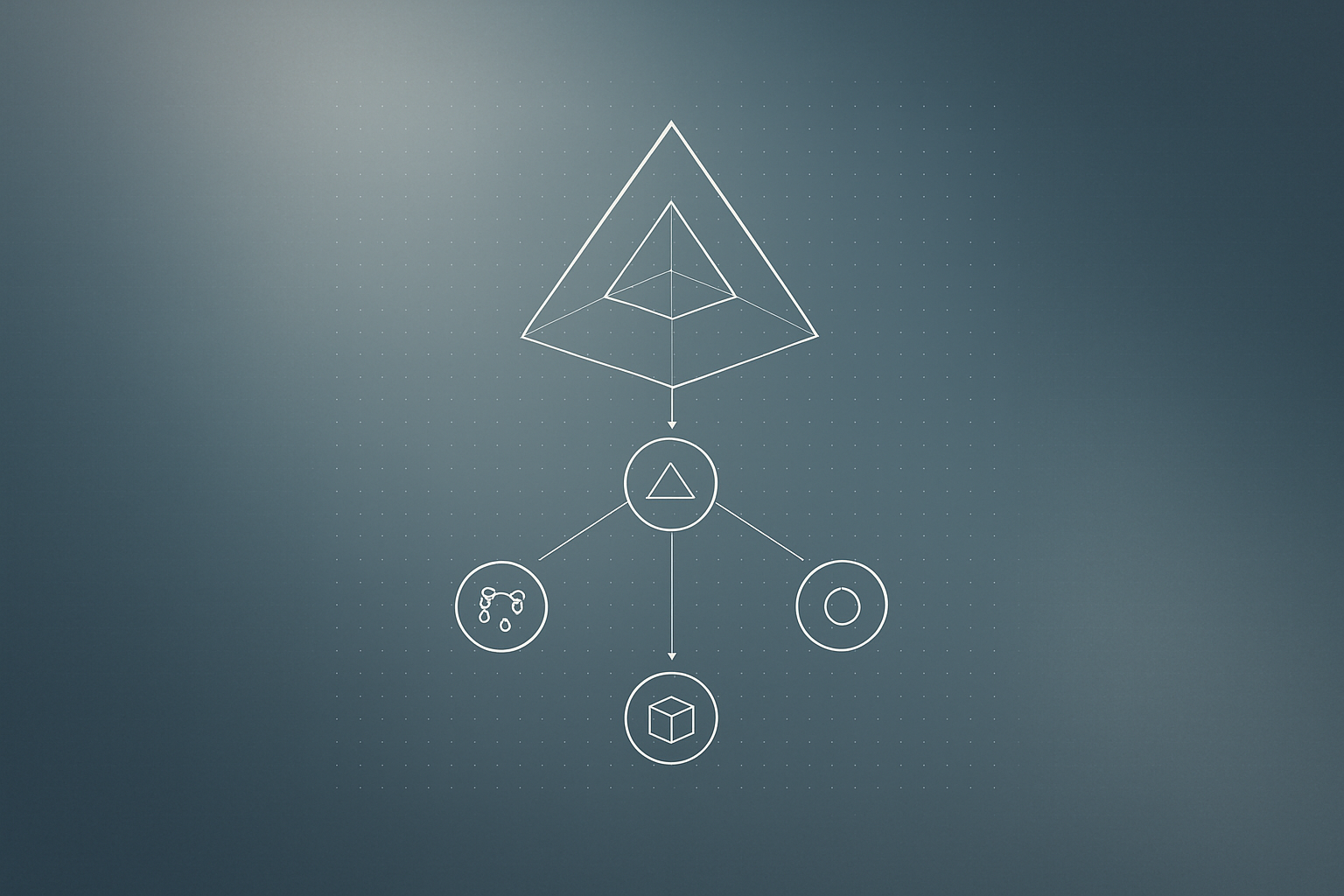
A new end-to-end tutorial published by Marktechpost walks through building a hierarchical Neural Radiance Field (NeRF) using JAX, Flax, Optax, and Google's JAX3D library. The pipeline covers synthetic multi-view dataset generation, a two-stage coarse-and-fine network with hierarchical importance sampling, JIT-compiled training with Adam and exponential learning-rate decay, and final evaluation through PSNR scoring, depth visualisation, and marching-cubes geometry extraction. It is aimed at researchers and engineers who want a working, GPU-adaptive NeRF implementation they can run today.

What happened

The tutorial assembles every piece of a production-grade NeRF in a single notebook. It pulls volume-rendering primitives directly from Google’s open-source jax3d repository, loading the volume_rendering.py module without triggering the full package’s heavy dependencies (gin, TensorFlow Data, etc.).

Config parameter	GPU value
Image resolution	64 x 64 px
Training views	24
Test views	3
Coarse samples per ray	64
Fine samples per ray	64
Network width / depth	128 units / 6 layers
Training steps	2,500
Initial learning rate	5e-4
Final learning rate	5e-6
Batch size (rays)	2,048
Geometry grid resolution	96

When no GPU is detected, the code automatically drops to a CPU-friendly config: 40 x 40 images, 14 training views, 400 steps, and a 64-unit wide network with only 4 layers.

How the pipeline is structured

Camera and ray setup

Cameras are placed on a dome using golden-angle azimuths paired with monotone elevations, which spreads views evenly without clustering. Each camera-to-world matrix is built with a standard look-at function following OpenGL/NeRF conventions (x right, y up, camera looking down -z). Rays are generated using pinhole intrinsics derived from a 40-degree field of view, with directions normalised to world-space unit length so that JAX3D’s depth samples map directly to real distances.

Coarse and fine networks

The NeRF model has two separate Flax networks. The coarse network samples 64 points uniformly along each ray. Those samples feed into hierarchical importance sampling via JAX3D’s sample_piecewise_constant_pdf, which draws an additional 64 fine samples concentrated where the coarse network predicts high density. Both networks share the same architecture: positional encoding with 10 frequencies for position and 4 frequencies for view direction, 6 fully connected layers of width 128, and a skip connection at layer 3.

Training setup

The tutorial uses JAX’s JIT compilation to keep the training loop fast, Adam optimisation via Optax, exponential learning-rate decay from 5e-4 down to 5e-6 over 2,500 steps, and gradient clipping to stabilise early training.

How does the tutorial evaluate novel-view synthesis?

Evaluation covers several angles rather than just a single number. PSNR (peak signal-to-noise ratio, a standard measure of image fidelity) is the primary metric. The tutorial also produces depth maps, opacity visualisations, sampling diagnostics, a full 360-degree render pass, and a marching-cubes mesh extraction from the trained density field at a grid resolution of 96.

Why it matters

NeRF is increasingly relevant beyond academic research. E-commerce teams use it for product visualisation, architecture firms use it for site walkthroughs, and game studios use it for asset capture. Tutorials like this one lower the barrier to shipping those applications because they skip the multi-library install hell that usually gates access to JAX3D’s primitives. If you are building a 3D product configurator or any experience that needs photorealistic novel views from a small set of photos, this is exactly the kind of toolchain worth understanding.

The hierarchical coarse-to-fine structure is also the right approach for production: you spend compute budget on the parts of the scene that actually have geometry, rather than sampling blank air uniformly. That detail matters when you move from a 64 x 64 toy scene to a real product at usable resolution.

Our take

This tutorial is solid reference material, but be honest about where it sits: a 64 x 64 synthetic scene at 2,500 steps is a proof-of-concept, not a pipeline you can drop on a real product shoot. The interesting engineering starts when you scale resolution, add real-world camera poses from COLMAP, and deal with unbounded scenes. The code structure here, particularly the clean separation of coarse and fine networks and the adaptive CPU/GPU config, is worth borrowing for a real project even if you end up replacing JAX3D’s primitives with something more maintained. Teams exploring AI-powered 3D tools as part of a broader AI integration strategy should treat this as a readable foundation, not a production-ready SDK. Check what the jax3d repo’s maintenance status looks like before building anything customer-facing on top of it.

What to do about it

1. Clone the google-research/jax3d repo at depth 1 and confirm the volume_rendering.py path exists before wiring anything else.
2. Run the CPU config first (no GPU required) to verify the full pipeline end-to-end before spending cloud compute credits.
3. Swap the synthetic analytic scene for your own multi-view photo set and real camera intrinsics once the toy version passes.
4. Profile PSNR at increasing resolutions to find where the coarse sample count (currently 64) becomes the bottleneck before tuning the fine network.
5. Evaluate marching-cubes output quality at grid resolution 96 against your target use case. Raise it if the mesh is too blocky, but expect memory cost to scale cubically.

If you want to ship 3D reconstruction to end users rather than just study the technique, pair this research baseline with a proper scene-capture workflow and keep an eye on newer NeRF variants (Instant NGP, 3D Gaussian Splatting) that train orders of magnitude faster.

Source: Marktechpost