Build a Batched Ensemble Weather Forecaster with NVIDIA Earth2Studio
A step-by-step look at building a custom batched ensemble weather forecasting pipeline with NVIDIA Earth2Studio, FCN, GFS data, and Zarr storage.
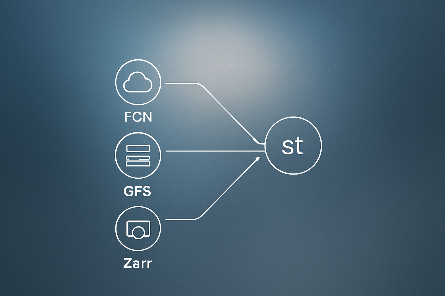
A new tutorial from Marktechpost walks through building a fully custom ensemble weather forecasting pipeline on top of NVIDIA Earth2Studio. The workflow loads the FCN prognostic model, pulls atmospheric initial conditions from NOAA's GFS, runs 8 ensemble members in batches of 2 across 8 forecast steps, and stores outputs in a Zarr data store. It also adds a custom wind-power diagnostic that converts 10-metre wind speed into turbine capacity factors, useful for renewable energy planning.
What happened
| Parameter | Value |
|---|---|
| Framework | NVIDIA Earth2Studio |
| Prognostic model | FCN (FourCastNet) |
| Atmospheric data source | NOAA GFS |
| Ensemble members (NENSEMBLE) | 8 |
| Batch size (BATCH_SIZE) | 2 |
| Forecast steps (NSTEPS) | 8 |
| Saved variables | t2m, z500, u10m, v10m, tcwv |
| Verified variables | t2m, z500, u10m |
| Point of interest | New Delhi (28.61N, 77.21E) |
The tutorial targets Google Colab and installs Earth2Studio with the fcn, data, perturbation, and statistics extras. Installation uses a constraint file that pins the existing Colab PyTorch and NumPy versions, so the CUDA environment survives the install. A GPU is strongly recommended: the code itself warns that a CPU runtime “will be very slow.”
How the pipeline works
Perturbation: noise that respects physics
The VariableScaledNoise class generates spatially correlated noise with per-variable amplitude settings. It tries to use Earth2Studio’s SphericalGaussian sampler first, falling back to Brown noise if that fails. Member zero is always kept clean as a control, so the ensemble contains one unperturbed run plus seven perturbed runs.
Custom diagnostic: wind to electricity
The WindPowerCF module takes the u10m and v10m wind components at 10 metres and converts them to a turbine capacity factor between 0 and 1. It extrapolates wind speed to hub height (default 100 metres) using a power-law shear exponent of 0.143, then applies a cubic ramp between a cut-in speed of 3 m/s and a rated speed of 12 m/s. The turbine is treated as fully on up to the cut-out speed of 25 m/s and off beyond that. This makes the forecast directly useful for renewable energy operations, not just meteorology.
Execution and storage
The pipeline uses Earth2Studio’s low-level iterator, coordinate-mapping, and batching APIs rather than its high-level runner. Forecast fields and diagnostic outputs are written to a Zarr backend, a chunked array format that preserves coordinate metadata alongside the data. This makes it straightforward to reload and slice results without re-running the model.
How forecast quality is measured
Verification runs against GFS analyses using four metrics:
- Latitude-weighted RMSE: standard error adjusted for the shrinking grid spacing near the poles.
- Fair CRPS (Continuous Ranked Probability Score): a proper scoring rule for probabilistic forecasts that rewards calibration, not just sharpness.
- Ensemble spread: the standard deviation across members, showing how much the ensemble disagrees.
- Spread-skill ratio: ideally close to 1.0, confirming the spread correctly predicts the error magnitude.
Visualisations include spatial uncertainty maps, geopotential-height spaghetti contours (one line per member), point-based fan charts for New Delhi, wind capacity factor forecasts, and lead-time skill curves showing how accuracy degrades with forecast horizon.
Why it matters
Most AI weather tutorials stop at a single deterministic forecast. Ensemble forecasting, running many slightly different initial conditions to sample forecast uncertainty, is how operational meteorology has worked for decades. This tutorial brings that approach into the Python/PyTorch world with a reproducible, open pipeline.
The wind-power diagnostic is the more commercially interesting addition. A capacity factor output lets energy traders, grid operators, or site planners query the model directly for business decisions rather than translating raw wind speeds themselves. The same pattern, wrapping a domain diagnostic inside the Earth2Studio coordinate system, works for solar irradiance, demand forecasting, or agricultural metrics.
For teams already using AI in operations, this is a worked example of how to attach custom business logic to a foundation model without retraining it. That pattern shows up in a lot of AI integration work we do for clients: the model stays frozen, the custom layer on top handles the domain-specific conversion.
Our take
The tutorial is technically solid and unusually honest about limitations (the CPU warning, the install constraint file). The code is longer than a blog post can fully show, but the architecture decisions are clear: use the low-level API, keep the control member, write to Zarr, verify against ground truth.
The wind-power diagnostic is the headline feature for business readers. It demonstrates that Earth2Studio’s coordinate system is flexible enough to bolt on arbitrary physics-informed post-processing. The catch is that this pipeline still requires a GPU and enough VRAM to run FourCastNet, which puts it out of reach for small teams without cloud compute. Running 8 members across 8 steps on a T4 will take real time.
If you are evaluating whether AI-driven weather data belongs in your product, start by asking what your current data source costs and how fresh it is. GFS is free and runs four times a day. A custom diagnostic on top of a free model, as shown here, can replace paid API calls for many operational use cases. We cover related developments in our AI news coverage and have shipped similar model-plus-diagnostic patterns for clients.
What to do about it
- Check whether your Colab runtime has a T4 or better before running: the notebook will not be fast otherwise.
- Fork the constraint-file install pattern for any Earth2Studio project that shares a Colab environment with other packages.
- Adapt
WindPowerCFto your site by changing hub height, cut-in, rated, and cut-out speeds to match your turbine spec sheet. - Monitor the spread-skill ratio. If it is well below 1.0, your perturbation amplitudes are too small and the ensemble is overconfident.
- Replace the GFS initial condition with a higher-resolution regional model if you need finer spatial detail for a specific geography.
The pattern here, a frozen foundation model plus a thin domain diagnostic, is the practical starting point for most operational AI weather integrations.
Frequently asked questions
What is NVIDIA Earth2Studio?
Earth2Studio is an open-source Python framework from NVIDIA for building AI-driven weather and climate forecasting workflows. It provides pre-trained prognostic models like FCN, data connectors for sources like GFS, perturbation tools, and a coordinate-aware I/O system.
What is ensemble weather forecasting and why does it matter?
Ensemble forecasting runs multiple slightly different versions of the same forecast to sample uncertainty. Instead of a single prediction, you get a spread of outcomes. Metrics like CRPS and spread-skill ratio tell you how well-calibrated that uncertainty is.
How does the wind power capacity factor diagnostic work in Earth2Studio?
The WindPowerCF module takes 10-metre u and v wind components, extrapolates to hub height using a power-law shear exponent of 0.143, then applies a cubic ramp between cut-in (3 m/s) and rated (12 m/s) speeds, capping at 1.0 up to the cut-out speed of 25 m/s.
What hardware do you need to run Earth2Studio FCN ensemble forecasts?
A CUDA-capable GPU is strongly recommended. The tutorial targets Google Colab with a T4 GPU. Running on CPU is possible but described in the code as very slow, especially for 8-member ensembles across 8 forecast steps.